Flowcharting in Excel Series
How to Create a Flowchart in Excel
By Nicholas Hebb
This article gives an overview on how to create flowcharts in Excel. There are significant differences between the tools in the newer versions of Excel and the older versions. Make sure that you read the appropriate section below. Most of the editing techniques are the same and are covered in the Editing Excel Flowcharts section at the bottom of the article. Most of the topics described here can also be applied to creating flowcharts in Word or PowerPoint, but in my humble opinion, of all the Office Drawing tools the Excel drawing tools are the most user friendly.
Excel Flowchart Wizard
FlowBreeze is a flowchart add-in for Microsoft Excel that makes creating flowcharts simple and pain free. Free 30-Day Trial.Setting Up The Environment
Before actually creating the flowchart, we will cover some preliminaries that make flowcharting in Excel a bit easier.
Creating a Grid (Optional)
A grid is not required, but it makes creating flowcharts with uniform shape sizes easier, especially when coupled with the Snap to Grid feature, which we will cover in the next section.
The grid is created by changing the column widths to match the standard row height. Assuming that you're using the default font of Calibri 11, the standard row height is 15 pts, which equals 20 pixels. To create the grid, change the column widths to 2.14 (= 20 pixels). (In case you're curious, the units for Excel column widths are based on the average number of characters that will fit within a cell.)
Follow the steps as described below these images:
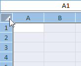
Click on the top left corner of the spreadsheet.
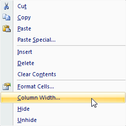
Right-click on any column and click on "Column Width".
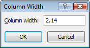
Enter 2.14 in the dialog and click OK.
Enabling Snap
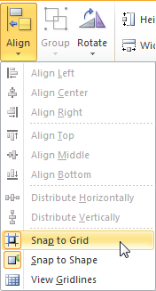
When Snap to Grid is turned on, anytime you add, move, or resize a shape, the edges of the shape will "snap" to the nearest grid line. Snap to Shape provides the same behavior, except shapes are snapped to the edges of other shapes. You can turn on both Snap to Grid and Snap to Shape by clicking the Page Layout tab, then click the Align dropdown, as shown in the image on the right.
Snap to Grid / Shape
Page Layout
Beyond the obvious reasons, setting the page layout before creating the flowchart is important for several reasons:
- If you plan to copy the flowchart from Excel to Word, or some other application, matching the margins to the target is important. Word, for example, has different normal margins than Excel.
- If the flowchart direction is left to right, the page layout is typically in landscape orientation.
- When you display page breaks, they act as a visual boundary to check whether shapes fall within a page.
To set the layout, click the Page Layout tab and use the Margins, Orientation, and (paper) Size dropdowns to change the settings if needed.
Themes: Be careful changing the Theme on the Page Layout tab. It not only alters the font and color scheme, but it also changes the row heights and column widths, which will affect how many shapes fit on a page.
Creating the Flowchart
Inserting a Flowchart Shape
To add the first shape, starting by clicking the Insert tab, where you should see a Shapes dropdown button. Clicking the Shapes dropdown displays the gallery of shape types shown below.
You can add a shape to the worksheet either by double-clicking a shape in the gallery, or by single clicking a shape and drawing its outline on the worskheet while holding the left mouse button down. If you double-click to add the shape, the shape will be placed in a somewhat arbritrary location on the sheet and have a height of 0.67" and a width of 1.0".
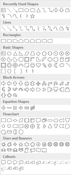
Insert Shapes Gallery
Adding More Flowchart Shapes
After you add the first shape, you'll notice that a Format tab (shown below) becomes available on the ribbon anytime that you click on a shape. We'll cover formatting in a bit, but in regard to adding shapes, the Format tab duplicates the Shapes gallery that we saw above. This makes it handy to add a shape then continue to add shapes in serial fashion.
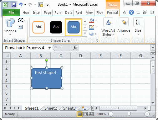
Format Tab
Adding Text to a Shape
This is straightforward - just click on the shape and start typing. If you need to edit the text in the shape click in the center of the shape, and not on the edges. Clicking the text in the center will put you into edit mode, but clicking the shape's border will select the shape itself.
Adding Connector Arrows Between Shapes
Connector arrows are added to the worksheet the same way flowchart shapes are - via the Shapes gallery. After clicking the line type in the gallery, follow these steps to add it to the flow diagram:
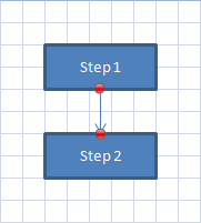
- Hover the mouse over the first shape and you will see the available connection points highlighted by red dots. Click the left mouse button down on the desired connection point.
- While still holding the left mouse bbutton down, drag the line to the next shape, where again the connection points are highlight.
- Release the left mouse button on a connection point, and the line will be selected with both end points highlighted by red dots. If an endpoint has a clear dot, it indicates that the connector wasn't connected.
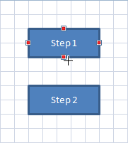
Insert connector - step 1
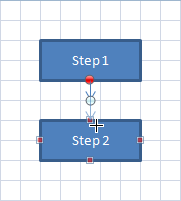
Insert connector - step 2
Insert connector - step 3
Adding Labels and Callouts
There are two common ways to add notes to a flowchart.
- Text box labels:

- Callouts:

Text boxes are often used to label the connectors coming out of decisions. Callouts are commonly used to add side comments, with their shape indicating that they are not a process step. Both can be added via the Insert Shapes gallery.
Formatting the Flowchart
There are so many formatting options in Excel, that it's too much to cover in a single article. The sections below show how to do basic shape and line formatting. There is a special dialog worth mentioning. If you right-click on a shape and select Format Shape from the context menu, the format dialog will display and let you make changes to a wide
Formatting Shapes
When one or more shapes is selected, the Format tab displays the style gallery shown below. Note that the styles changed in Excel 2013. The shape styles are set by their theme number, so if you use one of the purple styles in Excel 2010, for example, and then open it in Excel 2013, 2016, or 2019, it will display with the new orange theme.
If you are sharing the document with Excel 2003 users, note that the last row of styles will not render well in Excel 2003. If you are sharing the file with Excel 2000 users (i.e., the file is saved in .xls compatibility mode), the last two rows of styles will not render well.
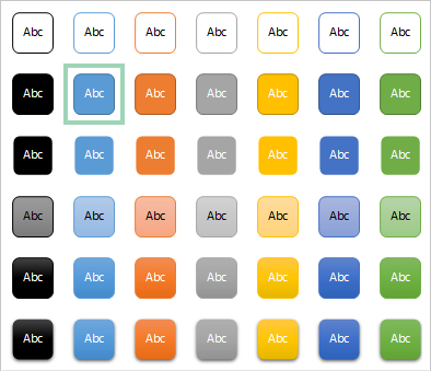
Excel 2013 - 2016 Shape Style Gallery
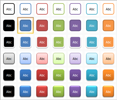
Excel 2007 - 2010 Shape Style Gallery
Formatting Connector Lines
When one or more connector lines is selected, the Format tab displays the line style gallery shown below. As with the shape styles, new line styles were also introduced in Excel 2013. Excel 2013 - 2019 lines are thinner and have no drop shadow. This is a good thing because the thicker lines and shadows were known to cause screen and print rendering problems.
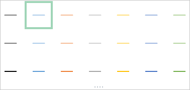
Excel 2013 - 2019 Line Style Gallery
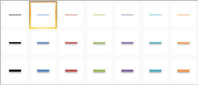
Excel 2007 - 2010 Line Style Gallery
Shape Fonts
Fonts are set for shapes the same way that they are for cells. Select the shape then set the font and font size on the Home tab.
Other Formatting Tips
- You can also use the Format Painter
 tool on the Home tab to quickly copy a format from one shape to another.
 - The Shape Fill dropdown lets you apply different fill colors and gradients and also allows you to insert a picture as a shape's background.
- The Shape Outline lets you change the line color, thickness, dash style, and arrow heads.
- The Shape Effects dropdown has a number of stylistics effects you can apply such as Shadow, Glow, Reflection, and more.
Editing the Flowchart
This section covers editing guidelines that are specific to Excel 2007-2010 only. For more tips that apply to all versions of Excel, scroll down to the Editing Excel Flowcharts section.
Selecting Shapes
The simplest way to select a single shape is to click on the border. You can select multiple shapes by holding the Ctrl key as you click. Once a shape is selected, you can toggle through the shape selections using the Tab key. Starting with Excel 2007, there is also a Selection Pane tool, accessible from the Format tab of the ribbon. The Selection Pane lists all the shapes by their names, not their text, so it isn't all that useful.
Aligning the Flowchart
If you created a grid and used Snap to Grid, hopefully you won't need to align any shapes after the fact, but in case you do, the Format ribbon tab has several features that are supposed to make this easier. under the Align dropdown menu, there are several options to align the selected shapes to the Left, Center, Right, etc. The left and rright alignment tools do what you would expect, but the centering tool moves all the shapes to the average center position, typically shifting all of them from their original position. As such, I typically recommend aligning shapes manually.
Changing a Flowchart Shape To Another Type
To change a shape, select it with your mouse, and then click on the Format tab. In the upper left, click the Edit Shape dropdown and select a new shape type, as shown in the image below. there is a bug in Excel 2007 and 2010 that you need to be aware of when using this tool. Changing a shape type causes any line connected to the shape to become unconnected. Connected lines will move with a shape when the shape is moved. Unconnected lines will not. Unconnected lines are also known to render strangely when printed or saved to PDF. In short, make sure to reconnect the lines after changing a shape type.

Edit Shape menu item
Setting Up The Environment
Enable the Drawing Toolbar
The first step to drawing flowcharts in Excel is to make the Drawing toolbar visible. This can be done by selecting View > Toolbars > Drawing from the main menu or by clicking the Drawing toolbar icon on the main Excel toolbar:

Create a Flow Chart Grid (Optional)
This step is optional, but it makes for a nicer flowcharting environment. To create a flow chart grid in Excel, select all the cells by clicking on the corner of the spreadsheet, as shown in the picture below-left. Then, right click on one of the columns and select Column Width. As shown in the picture below-right, enter 1.71 for the column width (which equals 17 pixels). The standard row height is 12.75 points, which also equals 17 pixels on most systems, so you get a nice tight square grid.
The standard row height is dependent on the default font. The default font in Excel 2000-2003 is Arial 10, so your settings may be different if you have a different font set as default.
Select all Excel cells
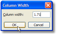 Set column width
Enable The Excel Snap to Grid Feature (Recommended)
This isn't required, but turning on the snap to grid function makes flowcharting in Excel so much easier I can't imagine creating flow charts without it. This feature makes the shapes align to the Excel worksheet cells when you add them, re-size them, or move them. It's great for ensuring your flowchart symbols are uniformly sized and aligned.
To turn snap to grid on, simply click the Draw button on the Drawing toolbar. Then, click Snap then To Grid, as shown below.
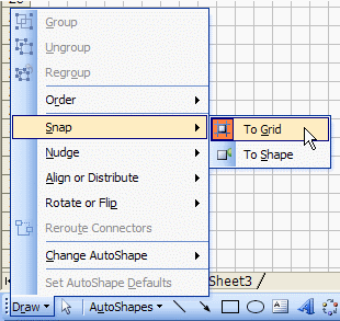
Excel Drawing toolbar - snap to grid
Set the Page Size and Boundaries
It's always good to know your limits, and making flow charts is no exception. You need to set the page size and then do a print preview because this will display the page breaks.
To setup the page properties, click File > Page Setup... from the main menu. Set properties such as portrait or landscape, paper size, and margins and close the form. One consideration you should make when setting the properties is where the flow chart will be published. For example, if you copy and paste the flow chart into Word, then it's good to remember that Word's default lateral page margins are 1" less than Excel's (i.e., 1/2" on both the left and right sides).
After the page properties are set, click the Print Preview button on the main toolbar. Alternately, you can click File > Print Preview from the menu. Close the preview screen and the page breaks should now be visible. If there is nothing on the worksheet yet to preview, Excel will pop open an error message. If it does, just click OK - the page breaks should now be visible anyway.
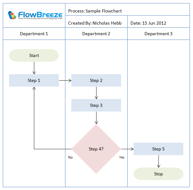
Create the Flow Chart Swim Lanes and Title Block (Optional)
If you're creating a Deployment Flow Chart, an Opportunity Flow Chart, a Process Relationship Flow Chart, or any other type of flow chart that requires swim lanes or swimming pools, then it's a good idea to create the structure of the flow chart before adding the flow chart symbols.
A full explanation of each of these specialized types of flow charts deserves an article of its own. But quickly, you can create the flow chart column and row headers in two ways. The first way is to use Excel's cell merging and borders. This is the easiest way if you plan on publishing the flow chart in Excel.
The second way is to create the headings with Process flow chart symbols and create the swim lane dividers with autoshape lines. The advantage to this method is that the swim lane heading shapes and dividing lines can be selected along with the flow chart symbols, so you can easily copy and paste the whole diagram if you're going to publish the flow chart in Word or some other Office application.
In the flow chart swim lane examples below, the swim lanes on the left were created using cell borders and the swim lanes on the right were created using process flow chart symbols and autoshape lines. As you can see, the appearance is identical.
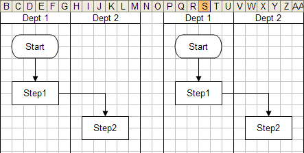
Swim lanes example
Also, if you plan to add a title block, including the process name, author(s), and revision info, then doing so before creating the flow chart is a good idea.
Add a Flow Chart Symbol
To add a flow chart symbol to the worksheet, you need to click the AutoShapes button on the Drawing toolbar, then click Flowchart, then select the shape you want to add, as shown in the picture below:
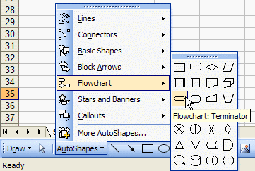
Excel flowchart autoshapes toolbar
The mouse cursor will change to a crosshair. Left click on the worksheet location where you want the top left corner of the flow chart symbol to be and drag the mouse until the flow chart symbol is the size you want. See the flow chart terminator symbol below for an example.
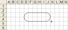
Add flowchart symbol example
Adding Text to a Symbol
To add text to an Excel flow chart symbol, simply click on the symbol and start typing. Note: If you've created Word flow charts before, this is one of the differences between creating flow charts in Excel and flow charts in Word. In Word, you have to right-click on the shape and select Add Text from the context menu.
Add a Connector (Flow Line) Between Two Symbols
[Note: A Flow Line is an arrow showing the order of the process steps. In Excel, flow chart lines are called Connectors. But Connector is also the name for a flow chart symbol used to depict a labeled node indicating a jump to another part of the flow chart. I will typically use the term "Flow Line" to avoid confusion, but in this section Flow Line and Connector are used interchangeably.]
Connectors are named as such because the lines actually connect to the flow chart shapes. When a shape is moved around, a Connector will remain attached to the shape, whereas a standard Excel line or arrow will not be connected.
To add a flow line between two shapes, first select the Connector type you want to use, as shown in the picture below. Tip: The Elbow Connector is versatile for flow lines because it will look just like a straight connector when the shapes are aligned.
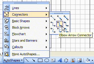
Excel Connectors toolbar
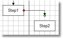
After you've clicked on a Connector type, the mouse will change to a crosshair. Click on the edge of the first flow chart symbol and drag the mouse over to the edge of the second flow chart symbol, then release the mouse button. A faint dashed line will show the path of the flow line. When you hover the mouse over a flow chart symbol, the possible connection points will show as blue dots. Also, the mouse cursor will change to a bomb site when you're near one of the connection points (see the picture below).
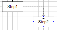
Adding connector arrows
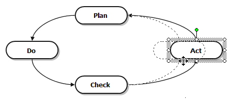
When an Excel flowchart Connector is connected to a flow chart symbol, the ends of the Connector are red dots. If one of the Connector ends is not connected it shows as a green dot. The figures below show a unconnected flow line on the left and a connected flow line on the right. To connect a flow line like this, just click and drag the endpoint to the correct spot.
Connector not attached to shape
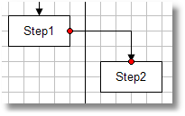
Connector attached to shape
A yellow diamond (not shown) on a Connector is a line routing handle. You can click and drag that to re-route the connector line without changing the position of the endpoints. It's a handy feature, especially when a long flow line is routed behind other shapes.
Adding Callouts
Sometimes you need to add a note or explanation for a flow chart process step that doesn't fit into the flow chart symbol. For these circumstances you can add a callout. Callouts are added from the Excel Drawing toolbar in the same way that you add a flow chart symbol or flow line.
Formatting Flow Chart Symbols
Many of the formatting features are available on the Excel Formatting toolbar (e.g., bold, italic, horizontal text alignment), and many others are available on the Excel Drawing toolbar (e.g., fill color, line color, line thickness, drop shadow).
Some of the formatting options are only available on the Format AutoShape dialog, such as vertical text alignment. This form can be opened by double-clicking on the outside border of the flow chart shape. Some of the more advanced formatting options are available in the Fill Effects sub-dialog, including gradient fills, textures, and adding pictures to flow chart symbols. The Fill Effects dialog is opened by clicking on the Fill Color dropdown as shown in the picture below.
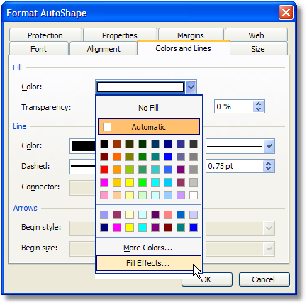
Format AutoShape dialog
Change a Flow Chart Symbol Type
Sometimes you decide a different flow chart symbol is needed. It's a common practice to make all shapes Process symbols (rectangles), but there's a lot of semantic information in symbols that conveys added meaning at-a-glance when you use more specific symbol types. To change a flow chart symbol type, first select the symbol. Then select the new shape from the Change AutoShape menu as shown below.
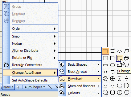
Change autoshape type
Aligning and Distributing Flow Chart Symbols
After you move or resize flow chart shapes, the alignment may get thrown off. Plus, if you resize a bunch of shapes to make them bigger, the spacing between the shapes may get scrunched up. Excel has a tool that can be found under the Draw menu on the Drawing toolbar to assist the Align or Distribute functions.
To use these functions, you must first select the shapes you want to align or distribute, then simply select the one of alignment (left, center, right, top, middle, bottom) or distribution (horizontally or vertically) functions to get the flow chart squared up. Alignment is self-explanatory, but distribution will take a set of shapes and spread out the distance between them uniformly.
Editing Excel Flowcharts
Move a Flow Chart Symbol
To move an Excel flow chart symbol, just click on the shape with your left mouse button and drag it to its new location. Excel will show dashed lines to preview the new layout, as shown below.
Move a flow chart symbol
You can also move a flow chart symbol with the arrow keys. Normally, the arrow keys will nudge the shape a small amount, but if the snap to grid feature is enabled, the arrow keys will move the flow chart symbol one cell at a time. To nudge a shape when snap to grid is enabled, hold the Control key down when you press the arrow key.
Resize a Flow Chart Symbol
First, Excel has an autosize feature available in the shape formatting dialog. Don't use it. Excel's idea of flow chart shape autosizing is to resize the shape so that all the text fits on one line.
Tip: You can move, resize, delete, or format multiple flow chart symbols at once. See this article on selecting multiple flow chart shapes .
To resize a flow chart symbol, first select the symbol by clicking on it with your mouse. The symbol will be highlighted and little circular handles will appear on the sides and corners, as shown in the picture below-left. Click and hold one of the handles and drag it in the direction that you want to resize the shape, as shown in the picture below-right. Excel will also display a dotted outline of the new shape size (not shown in the picture). Release the mouse button when the shape is the size you want.
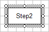
Selected Excel flow chart autoshape
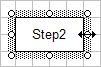
Resized Excel flow chart autoshape
Deleting Flow Chart Symbols
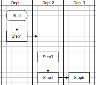
One of the least enjoyable things to do with a flow chart is maintain it. Here's a tip to make that process a little easier. Lets say you start with a flow chart that looks like this:
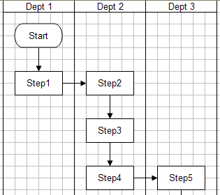
Delete shape - fig. 1
Delete shape - fig. 2
Delete shape - fig. 3
You want to delete Step 2, but that will leave a void, as shown above in fig. 2, which means, you have to move the other shapes. You can select multiple shapes using various methods and drag them to their new home. That works OK many times, but if the flowchart is really big it can be a hassle to select them and move them all.
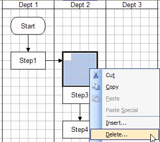
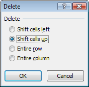
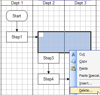
By default, Excel sets the flow chart autoshapes to move when cells are deleted, inserted, or resized. We can use this to our advantage by deleting cells to move the shapes. Select a range of cells as shown in the picture below. You must select a range of cell as wide or wider than the shapes you want to move! Right-click on the cells and select Delete... from the context menu. In the example, we want to move the shapes in this swim lane up, so we select Shift cells up, as shown in the image below.
Delete cells - Shift cells up
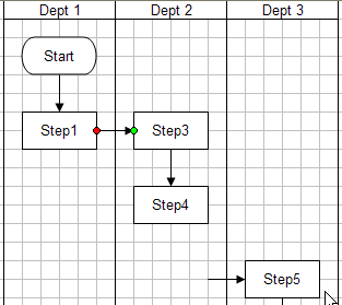
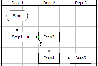
The result can be seen below in fig. 4. First there's the small issue of the flow line (Connector). It's not connected. Step 3 was moved into position to be connected to Step 1, but the connection still needs to be closed manually.
The second, and bigger, issue is the symbols in the Dept 3 swim lane. This method would have worked fine if there were only one swim lane. But the flowchart symbols in the Dept. 3 swim lane didn't get shifted. To remedy this we could have elected to delete the entire rows to have everything shift up. This option depends on the flow chart layout and what other shapes might be effected by such a move.
Delete shape - fig. 4
Delete shape - fig. 5
Delete shape - fig. 6
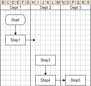
Another option would be to backtrack and select the cells from both the Dept 2 and Dept 3 swim lanes, as shown above in fig. 5, where we do a Delete... and Shift cells up, just as before. The result, in fig. 6, is much better. Now all you need to do is close the connection between Step 1 and Step 3.
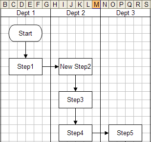
Inserting New Shapes Between Existing Shapes
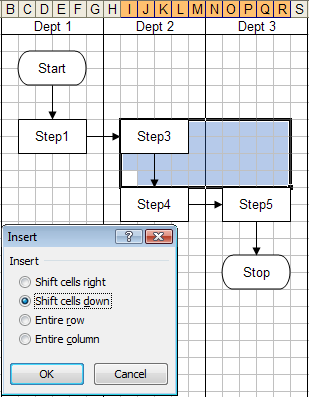
Inserting new flow chart symbols is essentially the same process as deleting a flow chart symbols - just in reverse. As with a Delete operation, we select the range of cells to perform the insert on. In fig. 1, the range is selected so that the cell shifting affects the other flow chart symbols in the desired way.
In fig. 2, a space has been opened up to place the new flow chart symbol, and in fig. 3, the new flow chart symbol has been added. Also, as shown in fig. 3, the connector from Step 1 is now connected to New Step 2, and a new connnector has been added between New Step 2 and Step 3.
Insert Excel shape - fig. 1
Insert Excel shape - fig. 2
Insert Excel shape - fig. 3
Miscellaneous Tips
- If you want to force line breaks at certain points in the text, hold the Alt key down when pushing the Enter key.
- The text inside the shape can be formatted (bold, italic, etc) using the standard formatting toolbar buttons.
- Autoshapes available from the Insert > Shapes gallery don't integrate directly with Smart Art shapes. Lines cannot be connected between them, and the formatting tools are separate.
- If shapes omit text when printed, try Grouping all the shapes before printing. This is a bug that exists since Excel 2007, and it is also seen with PDF creation and some print drivers.
Lastly, Excel is a great tool to create flowchart, and I hope this article was helpful to you. Most of the topics covered in this article can be automated using FlowBreeze, and, of course, as its creator, I encourage you to check it out.
About the Author
Nicholas Hebb
Nicholas Hebb is the owner and developer of BreezeTree Software, makers of FlowBreeze Flowchart Software, a text-to-flowchart maker, and Spreadspeed, an auditing and productivity toolset for Microsoft Excel®.